[Skip to Content](https://learning.oreilly.com/library/view/building-resilient-ip/1587052156/ch06.html#main) [](https://learning.oreilly.com/home/) - Explore Skills - Start Learning - Featured [Answers](https://learning.oreilly.com/answers2/) Search for books, courses, events, and more ## Chapter 6. Access Module --- This chapter covers the following topics: • [Multilayer Campus Design](https://learning.oreilly.com/library/view/building-resilient-ip/1587052156/ch06.html#ch06sec1lev1) • [Access Module Building Blocks](https://learning.oreilly.com/library/view/building-resilient-ip/1587052156/ch06.html#ch06sec1lev2) • [Layer 2 Domain](https://learning.oreilly.com/library/view/building-resilient-ip/1587052156/ch06.html#ch06sec1lev3) • [Layer 3 Domain](https://learning.oreilly.com/library/view/building-resilient-ip/1587052156/ch06.html#ch06sec1lev4) --- The access module is a network’s interface to the users or end stations, and challenges in the access module are often related to the physical or Layer 2 connectivity problems. Many Layer 2 technologies can be used to build the access module; however, the focus of this chapter is on the Ethernet technology because Ethernet has emerged as the _de facto_ connectivity standard for end devices. The ubiquity of the Ethernet technology lies in its simplicity and cost-effectiveness. The availability of Layer 3 switching technology brings IP and Ethernet together, and this has a profound impact on IP network design. For the first time, it is possible to build a complete network for an entire company using IP+Ethernet strategy, including workstation connections, servers in the data center, and connecting branches via a metro Ethernet offering from a service provider. The integration between IP and Ethernet here is so tightly coupled that problems found in the Layer 2 network directly impact the overall IP network availability. This chapter focuses on Ethernet switching technology, specifically Layer 2 network resiliency and how it should be built to provide a solid foundation for the Layer 3 network. ### Multilayer Campus Design With the popularity of Layer 3 switching, the term _multilayer campus design_ is almost synonymous with the Ethernet switching design. A multilayer campus design has two main characteristics: • **Hierarchical**—Each layer has a specific role to play. • **Modular**—The entire network is built by piecing building blocks together. These two characteristics enable the network to scale in a deterministic manner, with efficient use of resources to provide a resilient network foundation. 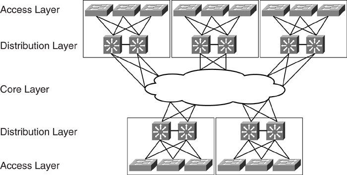[Figure 6-1](https://learning.oreilly.com/library/view/building-resilient-ip/1587052156/ch06.html#ch06fig01) shows the concept of a typical multilayer campus design. It has an access layer, which commonly consists of wiring closet switches. The access layer is connected to a distribution layer. The distribution layer is, in turn, connected to the core layer. From a high-level view, a group of access switches are connected to a pair of distribution switches to form a basic building block. Many of these building blocks exist within the network, and the core layer connects them. Designs such as this are also known as three-tier architecture. **Figure 6-1** _Three-Tier Multilayer Campus Design_  Note For the discussion on resilient IP networks, the access module in this chapter refers to the access and distribution layers in the multilayer campus design. The core module, which has been discussed in [Chapter 5](https://learning.oreilly.com/library/view/building-resilient-ip/1587052156/ch05.html#ch05), “[Core Module](https://learning.oreilly.com/library/view/building-resilient-ip/1587052156/ch05.html#ch05),” corresponds to the core layer. 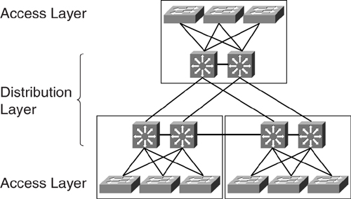Although [Figure 6-1](https://learning.oreilly.com/library/view/building-resilient-ip/1587052156/ch06.html#ch06fig01) shows a typical three-tier architecture, a smaller network may be built without the need of the core module at all, which makes it a two-tier design, as shown in [Figure 6-2](https://learning.oreilly.com/library/view/building-resilient-ip/1587052156/ch06.html#ch06fig02). **Figure 6-2** _Two-Tier Multilayer Campus Design_  The benefit of adopting the multilayer campus design is clarity of roles performed by each layer. The role of each layer is translated to a set of features required, which in turn translates to which particular type of hardware is to be used. #### Access Layer The access layer within the multilayer campus design model is where users gain access to the network. Most of the features found within the access layer are geared toward collecting and conditioning the traffic that is coming in from the users’ end stations. These features include the following: • Aggregating all the user endpoints • Providing traffic conditioning functions such as marking and policing • Providing intelligent network services such as automatic IP phone discovery • Providing network security services such as 802.1x and port security • Providing redundant links toward the distribution layer In the classic multilayer campus design, the access layer is mainly made up of Layer 2 switches. Therefore, most of the work done here is in optimizing the Layer 2 protocol that governs this layer. This helps to provide a robust Layer 2 environment for the functioning of the IP network. #### Distribution Layer The distribution layer within the multilayer campus design model aggregates the access layer. One of the most important characteristics of the distribution layer is that it is the point where the Layer 2 domain ends and where the Layer 3 domain begins. The features at the distribution layer include the following: • Aggregating access layer switches • Terminating virtual LANs (VLANs) that are defined within the Layer 2 domain • Providing the first-hop gateway service for all the end stations • Providing traffic conditioning services such as security, quality of service (QoS), and queuing • Providing redundant links toward the core layer, if required Because the distribution layer is the meeting place for both the Layer 2 and Layer 3 domains, it runs both Layer 2 and Layer 3 protocols. This is also the place where most of the network intelligence is found and is perhaps one of the most complex parts of the network. #### Core Layer The core layer within the multilayer campus design model has two important tasks: • Interconnect all the distribution layer blocks • Forward all the traffic as quickly as it can As the backbone of the entire network, its function is quite different from that of the access layer and distribution layer. The features that are critical to the functioning of the core layer include the following: • Aggregating distribution layers to form an interconnected network • Providing high-speed transfer of traffic among the distribution layers • Providing a resilient IP routing environment Because speed is of the essence here, the core layer usually does not provide services that may affect its performance (for example, security, access control, or any activities that require it to process every packet). In the discussion of multilayer campus design, the inclusion of a core layer is always an interesting question. For a small network, it is common to see a two-tier design, as shown earlier in [Figure 6-2](https://learning.oreilly.com/library/view/building-resilient-ip/1587052156/ch06.html#ch06fig02), for cost reasons. However, for bigger networks, inclusion of the core layer is always recommended to scale the network in a manageable fashion. 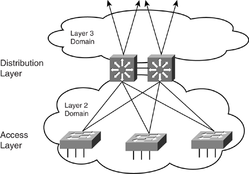### Access Module Building Blocks This section focuses on the individual building blocks shown in [Figure 6-3](https://learning.oreilly.com/library/view/building-resilient-ip/1587052156/ch06.html#ch06fig03). Making these individual building blocks rock solid is critical, because it is how the end users are connected to the network. These building blocks are to be found in the data center module, too, which you learn about in [Chapter 9](https://learning.oreilly.com/library/view/building-resilient-ip/1587052156/ch09.html#ch09), “[Data Center Module](https://learning.oreilly.com/library/view/building-resilient-ip/1587052156/ch09.html#ch09).” The well-being of an individual building block network relies on two factors: • How well the Layer 2 domain behaves within the building block • How its Layer 3 function interacts with the end devices and how well it is connected to the core layer **Figure 6-3** _Building Blocks for the Access Module_  The rest of this chapter describes the Layer 2 and Layer 3 domains. Within the Layer 2 domain, the focus is on resilient switching design, whereas the focus for the Layer 3 domain is on resilient IP services and routing design. ### Layer 2 Domain The access and distribution layers form the boundary for the Layer 2 domain of the building block network. This is an area where the Spanning Tree Protocol (STP) plays a critical role. Unfortunately, a common perception of STP is that it is a dated technology and has always been blamed for network disruptions. Whenever there is a network meltdown, chances are fingers will point toward the STP. The fact is, with proper design and configuration, STP is effective and useful. It is absolutely critical that in the access and distribution layers, a steady state of a Layer 2 network is a prerequisite for a stable IP network. You can have a well-designed IP network, but without a proper underlying Layer 2 network design, you will not be able to achieve your goal. Therefore, besides paying attention to the IP network design, you need to have a Layer 2 network strategy thought out. In addition, having a well-documented Layer 2 network is as essential as that of the Layer 3 network. Although STP was invented many years ago, it has been constantly improved to make it relevant in today’s networks. The next few sections help you understand the original protocol and the subsequent improvements made. These include the following: • [The Spanning Tree Protocol (IEEE 802.1d)](https://learning.oreilly.com/library/view/building-resilient-ip/1587052156/ch06.html#ch06sec2lev4) • [Trunking](https://learning.oreilly.com/library/view/building-resilient-ip/1587052156/ch06.html#ch06sec2lev5) • [Per-VLAN Spanning Tree (PVST)](https://learning.oreilly.com/library/view/building-resilient-ip/1587052156/ch06.html#ch06sec3lev9) • [Per-VLAN Spanning Tree Plus (PVST+)](https://learning.oreilly.com/library/view/building-resilient-ip/1587052156/ch06.html#ch06sec3lev10) • [802.1w](https://learning.oreilly.com/library/view/building-resilient-ip/1587052156/ch06.html#ch06sec2lev6) • [802.1s](https://learning.oreilly.com/library/view/building-resilient-ip/1587052156/ch06.html#ch06sec2lev7) • [Channeling technology](https://learning.oreilly.com/library/view/building-resilient-ip/1587052156/ch06.html#ch06sec2lev8) • [Best practices for the Layer 2 domain](https://learning.oreilly.com/library/view/building-resilient-ip/1587052156/ch06.html#ch06sec2lev9) #### The Spanning Tree Protocol: IEEE 802.1d The purpose of the STP, or IEEE 802.1d specification, is to prevent loops forming within a Layer 2 network. In a bridge network, looping causes problems such as broadcast storms. During broadcast storms, frames circulate in the network endlessly, consuming bandwidth and control plane resources. In a bridge network, there can only be one active path between two end stations that are communicating with one another. Note For the discussion on STP and its related features, the word _bridge_ is used, although the actual device you will be using is more likely a _switch_. 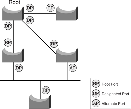Essentially, the STP uses the spanning-tree algorithm to keep track of redundant paths, and then chooses the best one to forward traffic while blocking the rest to prevent loops. The result of the STP is a tree with a root bridge and a loop-free topology from the root to all other bridges within the network. A blocked path acts as a backup path and is activated in the event that the primary path fails. Each of the ports on a bridge may be assigned a role, depending on the resulted topology: • **Root**—A forwarding port elected for the spanning-tree topology. There is always only one root port per bridge, and it is the port leading to the root bridge. • **Designated**—A forwarding port elected for a LAN segment. The designated port is in charge of forwarding traffic on behalf of the LAN segment, and there is always only one designated port per segment. • **Alternate**—A port that is neither root nor designated. • **Disabled**—A port that has been shut down and has no role. Depending on the port role, each port on a bridge will either be in forwarding state or blocked. The result is a tree topology that ensures a loop-free environment. [Figure 6-4](https://learning.oreilly.com/library/view/building-resilient-ip/1587052156/ch06.html#ch06fig04) shows a sample of a STP topology and the resulted role of the ports on the bridges. 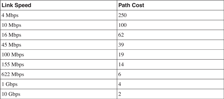**Figure 6-4** _Port Roles of STP_  Every bridge participating in a STP domain is assigned a bridge ID (BID) that is 8 bytes long. The BID is made up of a 2-byte bridge priority and a 6-byte Media Access Control (MAC) address of the switch. In addition, each of the bridge ports on the bridge is assigned a port ID. The port ID is 2 bytes long, with a 6-bit priority setting and a 10-bit port number. Each port also has a path cost that is associated with it. The original default path cost was derived by dividing 1 gigabit by the link speed of the port. However, with the introduction of higher-speed links such as the 10 Gigabit Ethernet, the default cost has been updated, as shown in [Table 6-1](https://learning.oreilly.com/library/view/building-resilient-ip/1587052156/ch06.html#ch06tab01). **Table 6-1** _Default Path Cost for STP_  Note You can also overwrite the default path cost with your own. However, it is always recommended that you keep the default values. The formation of the spanning tree is determined by the following: • The election of a root bridge • Calculating the path cost toward the root bridge • Determining the port role associated with each of the interfaces on the bridge The election of the root bridge is an important event in the STP and has a direct bearing on eventual traffic flow. Therefore, it is important for network designers to understand the concept of the election of the root and its impact on the network. The bridge with the lowest BID is always elected as a root bridge. Remember, BID is made up of the bridge priority and the MAC address. The default value of the bridge priority is 32768. Therefore, by default, the bridge with the lowest MAC address is usually elected as the root bridge. The root bridge acts like the center of a bridge network, and all traffic flows toward it. The paths toward the root that are deemed redundant are put in a blocked state. The STP is a timer-based protocol. As such, as a participant within the STP, a port goes through a series of states, based on some configured timing, before it starts to forward traffic. The cycle that a port goes through is reflected in [Figure 6-5](https://learning.oreilly.com/library/view/building-resilient-ip/1587052156/ch06.html#ch06fig05). 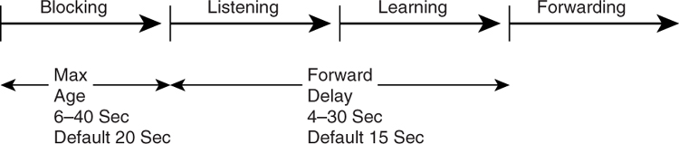**Figure 6-5** _The STP Cycle_  The states shown in [Figure 6-5](https://learning.oreilly.com/library/view/building-resilient-ip/1587052156/ch06.html#ch06fig05) are as follows: • **Blocking**—No traffic is forwarded. • **Listening**—First state whenever a port is first initialized. In this state, the bridge is trying to determine where the port fits in the STP topology. • **Learning**—The port gets ready to forward traffic. In this state, the port is trying to figure out the MAC address information that is attached to the port. • **Forwarding**—The port is forwarding traffic. • **Disabled**—The port has been disabled. In the discussion of optimizing a switched network, three parameters are of utmost importance: • **Hello timer**—Determines how often a bridge sends out BPDUs • **Forward delay timer**—Determines how long the listening and learning states must last before a bridge port starts forwarding traffic • **Maximum age timer**—Determines the length of time a bridge stores its information received As you can see in [Figure 6-5](https://learning.oreilly.com/library/view/building-resilient-ip/1587052156/ch06.html#ch06fig05), the time taken for transiting from power up to start of transmission for a bridge port is at least 35 seconds. That is, no IP traffic can be transmitted for at least that amount of time. Obviously, if the port goes up and down in a span of 35 seconds, no traffic actually flows through it. 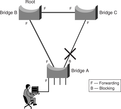[Figure 6-6](https://learning.oreilly.com/library/view/building-resilient-ip/1587052156/ch06.html#ch06fig06) shows a simple setup of three bridges connected together. After the STP has converged, the resulted topology is as shown with bridge B being selected as the root bridge. The link between bridge A and C is blocked to prevent a loop. **Figure 6-6** _STP in Steady State_  The following sections discuss various scenarios that can happen to this steady-state network. The behavior of STP is studied and suggestions are made on how to improve its capability to react to problems. The following features within the Catalyst series of switches are highlighted in the discussion of how to overcome problems: • [PortFast](https://learning.oreilly.com/library/view/building-resilient-ip/1587052156/ch06.html#ch06sec3lev1) • [UplinkFast](https://learning.oreilly.com/library/view/building-resilient-ip/1587052156/ch06.html#ch06sec3lev2) • [BackboneFast](https://learning.oreilly.com/library/view/building-resilient-ip/1587052156/ch06.html#ch06sec3lev3) • [Unidirectional Link Detection (UDLD)](https://learning.oreilly.com/library/view/building-resilient-ip/1587052156/ch06.html#ch06sec3lev4) • [RootGuard](https://learning.oreilly.com/library/view/building-resilient-ip/1587052156/ch06.html#ch06sec3lev5) • [LoopGuard](https://learning.oreilly.com/library/view/building-resilient-ip/1587052156/ch06.html#ch06sec3lev6) • [BPDUGuard](https://learning.oreilly.com/library/view/building-resilient-ip/1587052156/ch06.html#ch06sec3lev7) ##### PortFast As described in the preceding section, a port usually takes about 35 seconds before it starts to forward traffic. In some instances, this behavior is undesirable. One example is when an end station is connected to the port. Because the port takes 35 seconds to begin forwarding traffic, the following errors may potentially occur: • If the end station is running a Windows client, it may encounter the error “No Domain Controllers Available.” • If the end station is trying to request an IP address via a Dynamic Host Configuration Protocol (DHCP) server, it may encounter the error “No DHCP Servers Available.” • If the end station is running the Internetwork Packet Exchange (IPX) protocol, it may encounter no login screen. The errors may occur for a few reasons, such as a link-speed negotiation problem or duplex problems. However, the way the STP port behaves may have contributed to the problem. One of the reasons errors occur is that the port is still transiting to the forwarding state even after those protocol requests have been sent out by the end station. This is not uncommon, because advancement in end station technology has resulted in extremely fast boot time. The booting of the operating systems is so fast now that the system sends out requests even before the port goes into a forwarding state. As shown in the STP topology illustrated earlier in [Figure 6-6](https://learning.oreilly.com/library/view/building-resilient-ip/1587052156/ch06.html#ch06fig06), user-facing ports are connected to end stations only. These ports do not connect to other bridges and are called _leaf nodes_. The use of the STP is to prevent loops between bridges. Therefore, there is no reason why a leaf node needs to toggle through the different states, because it will not be connecting to another bridge. It might be possible to bypass those transition states and put the port into forwarding mode immediately upon detection of a connection. The **portfast** command in the Catalyst series switches is a feature that enables a leaf node in the STP topology to have such bypass capability. It can be configured at the global level, in which all ports are configured with the PortFast feature by default. It can also be configured at the individual port level. It is critical that a port with the PortFast feature enabled should only be used for connection to end devices. It should never be connected to other Layer 2 devices such as a hub, switch, or bridge. For this reason, configuring the PortFast feature at port level is always preferred. [Example 6-1](https://learning.oreilly.com/library/view/building-resilient-ip/1587052156/ch06.html#ch06ex01) demonstrates how to configure the PortFast feature at the port level. 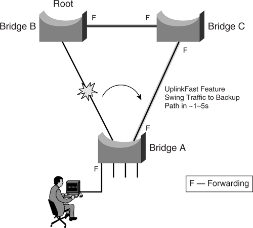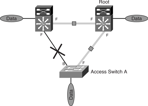**Example 6-1** _Configuring PortFast_ --- Cat3750#configure terminal Cat3750(config)#interface GigabitEthernet 1/0/1 Cat3750(config-if)#spanning-tree portfast --- ##### UplinkFast [Figure 6-6](https://learning.oreilly.com/library/view/building-resilient-ip/1587052156/ch06.html#ch06fig06) illustrated a simple Layer 2 network that is in steady state, with bridge A forwarding traffic toward bridge B. The link that is connected to bridge C is blocked and acts as a redundant link. By default behavior of STP, when the link between bridge A and B fails, the STP needs about 30 seconds before diverting traffic to the redundant link. Before the redundant link takes over, all user traffic from bridge A is not forwarded, as shown in [Figure 6-7](https://learning.oreilly.com/library/view/building-resilient-ip/1587052156/ch06.html#ch06fig07). 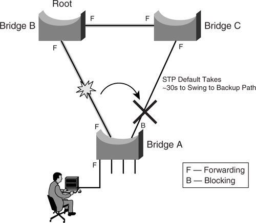**Figure 6-7** _Default STP Action on an Uplink Failure_  Because the backup link takes such a long time to forward traffic, one area of focus is how to accelerate the takeover process so that traffic is diverted to the redundant link immediately after the active link has failed. 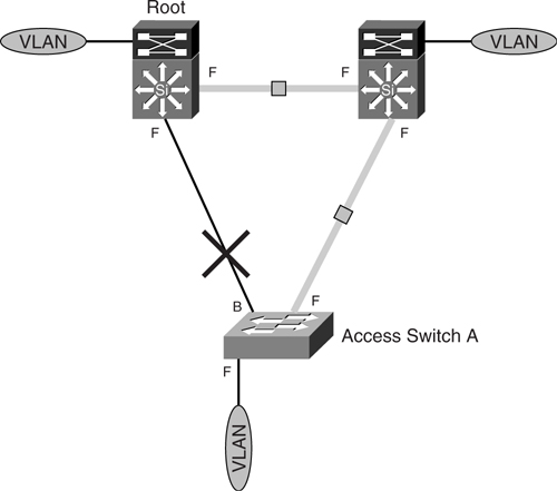The feature that makes this possible is delivered through the UplinkFast feature. Essentially, UplinkFast moves the original blocked port on bridge A to the forwarding state without going through the listening and learning states, as shown in [Figure 6-8](https://learning.oreilly.com/library/view/building-resilient-ip/1587052156/ch06.html#ch06fig08). **Figure 6-8** _STP Action with UplinkFast_  When the UplinkFast feature is enabled, the bridge priority of bridge A is set to 49152. If you change the path cost to a value less than 3000 and you enable UplinkFast or UplinkFast is already enabled, the path cost of all interfaces and VLAN trunks is increased by 3000. (If you change the path cost to 3000 or above, the path cost is not altered.) The changes to the bridge priority and the path cost reduce the chance that bridge A will become the root bridge. It is important to note that the UplinkFast feature is most applicable to access switches only and may not be relevant in other parts of the network. In addition, it is a feature that is most useful in a triangular topology, such as the one previously shown. Its behavior may not be so predictable in other complex topologies, as discussed later in the section “[Layer 2 Best Practices](https://learning.oreilly.com/library/view/building-resilient-ip/1587052156/ch06.html#ch06sec2lev9).” The **uplinkfast** command is issued at the global level. [Example 6-2](https://learning.oreilly.com/library/view/building-resilient-ip/1587052156/ch06.html#ch06ex02) shows an example configuration of the UplinkFast feature. **Example 6-2** _Configuring UplinkFast_ --- Cat3750#configure terminal Cat3750(config)#spanning-tree uplinkfast --- ##### BackboneFast In the steady-state network, sometimes links other than those connected directly to bridge A will fail, as shown in [Figure 6-9](https://learning.oreilly.com/library/view/building-resilient-ip/1587052156/ch06.html#ch06fig09). 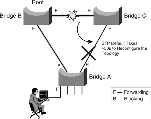**Figure 6-9** _Default STP Action Without BackboneFast_  An indirectly connected failure causes bridge A to receive a type of BPDU called an _inferior BPDU_. An inferior BPDU indicates that a link that is not directly connected to this bridge has failed. Under STP default configuration, bridge A ignores the inferior BPDU for as long as the maximum aging timer; therefore, the STP topology is broken for as long as 50 seconds. That means no traffic flow from bridge A for 50 seconds. 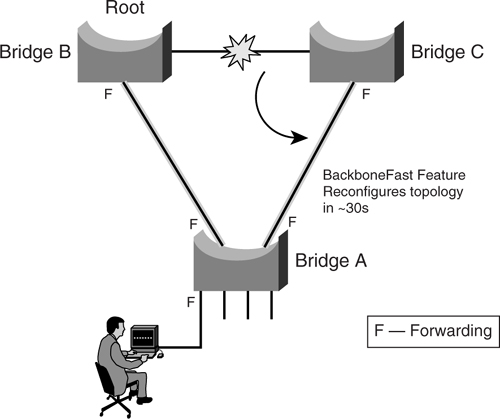The BackboneFast feature on bridge A circumvents this problem by initiating a state transition on the blocked port from blocked to listening state. This is done without waiting for the maximum aging time to expire and, thus, speeds up topology reconstruction to about 30 seconds, as shown in [Figure 6-10](https://learning.oreilly.com/library/view/building-resilient-ip/1587052156/ch06.html#ch06fig10). **Figure 6-10** _STP Action with BackboneFast_  The **backbonefast** command is issued at the global level. [Example 6-3](https://learning.oreilly.com/library/view/building-resilient-ip/1587052156/ch06.html#ch06ex03) shows an example configuration of the BackboneFast feature. **Example 6-3** _Configuring BackboneFast_ --- Cat3750#configure terminal Cat3750(config)#spanning-tree backbonefast --- ##### Unidirectional Link Detection (UDLD) Up to this point, all the features discussed deal with a link or box failure scenario. However, there is still a possibility of a physical error that may wreak havoc in the access module and that is a unidirectional link error. A unidirectional link occurs whenever traffic sent by a device is received by its neighbor, but traffic from the neighbor is not received by the device. This happens, especially with fiber cabling, when only part of the fiber pair is working. A unidirectional link error can cause unpredictable behavior from the network, especially with the STP topology. The situation depicted in [Figure 6-11](https://learning.oreilly.com/library/view/building-resilient-ip/1587052156/ch06.html#ch06fig11) does happen with fiber cabling systems that use a patch panel. In the figure, the switch ports are patched incorrectly at the patch panel, which may be located far away from the switches. The consequence of the erroneous cabling is unpredictable and may be difficult to troubleshoot just by issuing commands on the switch console. Even though the port status displays as up and working, errors will occur at the higher-layer protocol. In certain cases, the STP may still consider the link valid and move the effected port into a forwarding state. The result can be disastrous because it will cause loops to occur in the Layer 2 network. 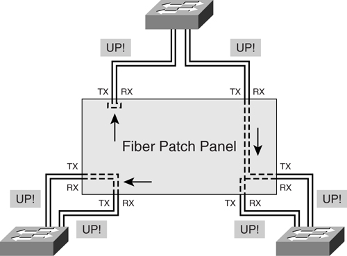**Figure 6-11** _Possible Causes of Unidirectional Link Error_  The UDLD feature provides a way to prevent errors such as the one depicted in [Figure 6-11](https://learning.oreilly.com/library/view/building-resilient-ip/1587052156/ch06.html#ch06fig11). It works with the Layer 1 mechanism to prevent one-way traffic at both physical and logical connections. The Layer 1 mechanism works by using the autonegotiation feature for signaling and basic fault detection. UDLD operates by having the devices exchange Layer 2 messages and detect errors that autonegotiation cannot. A device will send out a UDLD message to its neighbor with its own device/port ID and its neighbor’s device/port ID. A neighboring port should see its own ID in the message; failure to do so in a configurable time means that the link is considered unidirectional and is shut down. UDLD can be configured in two modes: • **Normal**—If the physical link is perceived to be up but UDLD does not receive the message, the logical link is considered undetermined, and UDLD does not disable the port. • **Aggressive**—If the physical link is perceived to be up but UDLD does not receive the message, UDLD will try to reestablish the state of the port. If the problem still persists, UDLD shuts down the port. Aggressive mode also supports detection of one-way traffic on twisted-pair cable. You can configure UDLD at both the global level and at the port level. [Example 6-4](https://learning.oreilly.com/library/view/building-resilient-ip/1587052156/ch06.html#ch06ex04) shows how to configure UDLD at the global level. **Example 6-4** _Configuring UDLD Globally_ --- Cat3750#configure terminal Cat3750(config)#udld enable --- [Example 6-5](https://learning.oreilly.com/library/view/building-resilient-ip/1587052156/ch06.html#ch06ex05) shows how to configure UDLD at the port level. **Example 6-5** _Configuring UDLD at the Port Level_ --- Cat3750#configure terminal Cat3750(config)#interface GigabitEthernet 1/0/1 Cat3750(config-if)#udld port --- ##### RootGuard If you are running STP, the resulting topology always centers on the location of the root bridge. Whether a particular physical link is used or not depends on the port state of either forward or blocked. And this, in turn, depends on the location of the root bridge. It is possible that a certain topology was envisioned during the design phase so that traffic flows in a certain direction. However, the introduction of an additional bridge may turn things around and have an unexpected result, as shown in [Figure 6-12](https://learning.oreilly.com/library/view/building-resilient-ip/1587052156/ch06.html#ch06fig12). 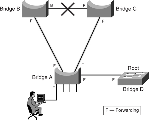**Figure 6-12** _Result of Illegal Root Bridge Introduction_  Before the introduction of the new bridge D, the topology of the network was intended as that shown earlier in [Figure 6-6](https://learning.oreilly.com/library/view/building-resilient-ip/1587052156/ch06.html#ch06fig06). However, the topology changes when bridge D is introduced. Because bridge D has a lower bridge priority, it begins to announce that it is the new root bridge for the Layer 2 topology. As a result, a new topology is formed to account for this new root bridge. As shown in [Figure 6-12](https://learning.oreilly.com/library/view/building-resilient-ip/1587052156/ch06.html#ch06fig12), the link between bridge B and bridge C has now been blocked. In other words, the communication path between the two bridges has to be via bridge A. If both links from bridge A are slow links, say 10 Mbps, this might have a performance impact between the two bridges B and C. The RootGuard feature prevents the preceding scenario from happening. It is configured on a per-port basis and disallows the port from going into root port state. [Example 6-6](https://learning.oreilly.com/library/view/building-resilient-ip/1587052156/ch06.html#ch06ex06) shows how to configure the RootGuard feature. **Example 6-6** _Configuring RootGuard_ --- Cat3750#configure terminal Cat3750(config)#interface fastethernet 1/0/24 Cat3750(config-if)#spanning-tree guard root --- In [Example 6-6](https://learning.oreilly.com/library/view/building-resilient-ip/1587052156/ch06.html#ch06ex06), when a BPDU that is trying to claim root is received on the port, it goes into an error state called _root inconsistent_. The new state is essentially the same as the listening state and will not forward traffic. When the offending device has stopped sending BPDU, or the misconfiguration has been rectified, it will go into a forwarding state again. This way, a new bridge cannot “rob” the root away from the Layer 2 network. The following shows the error message that appears if RootGuard is put into action: %SPANTREE-2-ROOTGUARDBLOCK: Port 1/0/24 tried to become non-designated in VLAN 10. Moved to root-inconsistent state To prevent the situation illustrated in [Figure 6-12](https://learning.oreilly.com/library/view/building-resilient-ip/1587052156/ch06.html#ch06fig12) from happening, you should introduce the RootGuard feature in bridge A on the port facing bridge D. ##### LoopGuard Even if STP is deployed, loops might still occur. Loops happen when a blocked port in a redundant topology erroneously transits to a forwarding state, which usually happens because one of the ports of a physically redundant topology (not necessarily the STP blocking port) stopped receiving BPDUs. As a timer-based protocol, STP relies on continuous reception or transmission of BPDUs, depending on the port role (designated port transmits, nondesignated port receives BPDUs). So when one of the ports in a physically redundant topology stops receiving BPDUs, the STP conceives that nothing is connected to this port. Eventually, the alternate port becomes designated and moves to a forwarding state, thus creating a loop. The LoopGuard feature was introduced to provide additional protection against failure, such as the one just described. With the LoopGuard feature, if BPDUs are not received any more on a nondesignated port, the port is moved into a new state, called the loop-inconsistent state. The aim is to provide a sanity check on the change in topology. [Example 6-7](https://learning.oreilly.com/library/view/building-resilient-ip/1587052156/ch06.html#ch06ex07) shows how to configure LoopGuard on all ports at the global level. **Example 6-7** _Configuring LoopGuard_ --- Cat3750#configure terminal Cat3750(config)#spanning-tree loopguard default --- The following shows the error message that appears on the console when an error is detected by LoopGuard: SPANTREE-2-LOOPGUARDBLOCK: No BPDUs were received on port 3/4 in vlan 8. Moved to   loop-inconsistent state. Note You cannot enable both the RootGuard and LoopGuard at the same time. ##### BPDUGuard BPDUGuard is a feature that is recommended to be run together with the PortFast feature. Remember that the PortFast feature allows a port that has end systems connected to it to skip various STP states and go directly into a forward state. The port is not supposed to be connected to other bridges and, therefore, should not be receiving BPDUs. Any detection of a BPDU coming from the port is an indication that an invalid bridge has been introduced into the Layer 2 network. Upon detection of a BPDU, the BPDUGuard feature sends the port immediately into an error-disabled state, which enables you to investigate the problem, and rectify the situation before disaster strikes. BPDUGuard can be enabled at the global command level as a global PortFast option. It can be also configured at the individual port level for granular control. [Example 6-8](https://learning.oreilly.com/library/view/building-resilient-ip/1587052156/ch06.html#ch06ex08) shows how to configure BPDUGuard. **Example 6-8** _Configuring BPDUGuard_ --- Cat3750#configure terminal Cat3750(config)#spanning-tree portfast bpduguard default --- #### VLANs and Trunking Thus far, the discussion has focused on a common bridged network. The advent of Layer 2 switching technology introduces many new concepts that require further understanding and treatment for STP. For example, with Layer 2 switching comes the concept of VLANs and trunking. A VLAN is basically a collection of network nodes that share the same broadcast domain. In a switched network design, an IP subnet is usually mapped to a VLAN, although there may be a rare exception. Because of their close association, the health of a VLAN directly impacts the functioning of the associated IP subnet. The introduction of a VLAN brings about the concept of trunking, when many VLANs have to be transported across a common physical link. [Figure 6-13](https://learning.oreilly.com/library/view/building-resilient-ip/1587052156/ch06.html#ch06fig13) shows the trunking process. 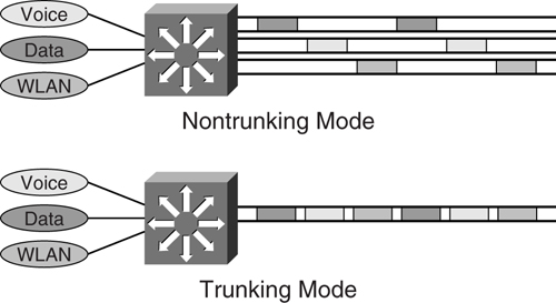**Figure 6-13** _Nontrunking Versus Trunking Mode_  The reason for using the trunking mode feature varies, but the most obvious one is to save on ports that would have otherwise been spent on carrying each individual VLAN. This is especially true when connecting an access switch to the distribution layer. To carry multiple VLANs across the single physical link, a tagging mechanism or encapsulation has to be introduced to differentiate the traffic from the different VLANs. There are two ways of achieving this: • Inter-Switch Link (ISL) • IEEE 802.1q ISL is a Cisco proprietary way of carrying different VLANs across a trunk. It is an encapsulation method whereby the payloads are wrapped with a header before transmission across the trunk. [Figure 6-14](https://learning.oreilly.com/library/view/building-resilient-ip/1587052156/ch06.html#ch06fig14) shows the format of an ISL frame. 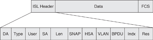**Figure 6-14** _ISL Header_  The fields in the ISL header are as follows: • **DA**—Destination address • **Type**—Frame type • **User**—User-defined bits • **SA**—Source address • **Len**—Length • **SNAP**—Subnetwork Access Protocol • **HAS**—High bits of source address • **VLAN**—Destination virtual LAN ID • **BPDU**—Bridge protocol data unit • **Indx**—Index • **Res**—Reserved ISL encapsulation adds 30 bytes to the original data frame. The implication of this is that you have to be careful of maximum transmission unit (MTU) size support on the various transmission interfaces. If the entire ISL-encapsulated frame size is bigger than the MTU size of the interface, fragmentation may occur. The largest Ethernet frame size with ISL tagging is 1548 bytes. Another point worth noting is that an ISL frame contains two Frame Check Sequence (FCS) fields: one for the original data frame, which is kept intact during encapsulation; and another one is for the ISL frame itself. Therefore, any corruption within the original data frame will not be detected until the ISL frame is de-encapsulated, and the original frame is sent to the receiver. ISL can carry up to 1000 VLANs per trunk. [Example 6-9](https://learning.oreilly.com/library/view/building-resilient-ip/1587052156/ch06.html#ch06ex09) shows how to turn on trunking on a switch port using ISL. **Example 6-9** _Configuring ISL Trunking_ --- Cat3750#configure terminal Cat3750(config)#interface fastethernet 1/0/24 Cat3750(config-in)#switchport mode trunk Cat3750(config-in)#switchport trunk encapsulation isl --- The other trunking mechanism is the IEEE 802.1q standard. It uses an internal tagging method that inserts a 4-byte Tag field into the original Ethernet frame. The Tag field is located between the Source Address and Type/Length fields, as shown in [Figure 6-15](https://learning.oreilly.com/library/view/building-resilient-ip/1587052156/ch06.html#ch06fig15). 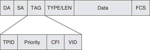**Figure 6-15** _IEEE 802.1q Tag Field_  The Tag field is as follows: • **TPID**—Tag protocol identifier • **Priority**—User priority • **CFI**—Canonical format indicator • **VID**—VLAN identifier For IEEE 802.1q tagging, there is only one FCS field. Because the frame is altered during the tagging, the FCS is recomputed on the modified frame. Because the tag is 4 bytes long, the resulting Ethernet frame size can be 1522 bytes. The IEEE 802.1q can carry 4096 VLANs. [Example 6-10](https://learning.oreilly.com/library/view/building-resilient-ip/1587052156/ch06.html#ch06ex10) shows how to turn on trunking on a switch port using 802.1q. **Example 6-10** _Configuring 802.1q Trunking_ --- Cat3750#configure terminal Cat3750(config)#interface fastethernet 1/0/24 Cat3750(config-in)#switchport mode trunk Cat3750(config-in)#switchport trunk encapsulation dot1q --- The 802.1q is the preferred method for implementing trunking because it is an open standard. In addition, 802.1q can carry more VLANs, a feature that is good to have in a metro Ethernet implementation. The implication of VLANs and trunking is not so much having the concept of multiple broadcast domains within a single device, or the ability to carry multiple VLANs across a single physical link. It is the concept of multiple instances of STP that comes with it that is crucial in resilient network design. The following sections show how to deal with this challenge. ##### Common Spanning Tree (CST) As discussed previously, the purpose of STP is to prevent loops from forming in a Layer 2 network. The introduction of the switch gives rise to many broadcast domains, called the VLANs. The IEEE 802.1d, as a protocol, does not have the concept of VLAN. The IEEE 802.q introduces the concept of VLANs, and it subjects the multiple VLANs to the control of a single STP instance by introducing a native VLAN that is not tagged during transmission. The STP state of the native VLAN governs the topology and the operation of the rest of the tagged VLANs. This mode of operation is commonly known as _Common Spanning Tree_ (_CST_). [Figure 6-16](https://learning.oreilly.com/library/view/building-resilient-ip/1587052156/ch06.html#ch06fig16) illustrates the concept of a CST. Because there is only one instance of STP, all the VLANs share the same topology, with common forwarding ports and blocked ports, depending on the final STP state. In this case, no load balancing of traffic is possible and the redundant path does not carry any user traffic during normal operation. 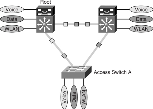**Figure 6-16** _Common Spanning Tree Topology_  ##### Per-VLAN Spanning Tree (PVST) In contrast to CST, the Per-VLAN Spanning Tree (PVST) is a Cisco proprietary extension of IEEE 802.1d. It introduces an instance of STP process for each VLAN being configured in the Layer 2 networks. In this manner, each VLAN may have a different topology, depending on individual STP configuration. PVST works only with ISL trunking. [Figure 6-17](https://learning.oreilly.com/library/view/building-resilient-ip/1587052156/ch06.html#ch06fig17) illustrates the concept of a PVST implementation. 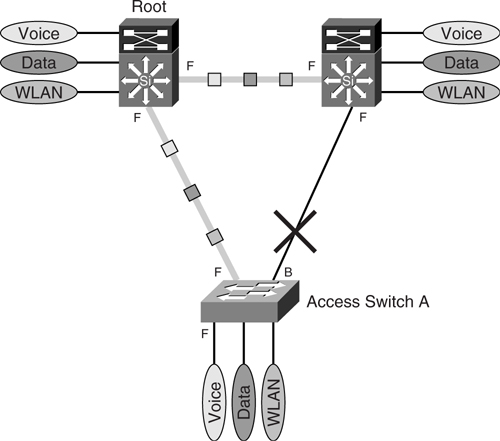**Figure 6-17** _PVST Topology_  Because there is one instance of STP per VLAN, each VLAN can have its own topology, independent of the others. [Figure 6-18](https://learning.oreilly.com/library/view/building-resilient-ip/1587052156/ch06.html#ch06fig18) shows the topology of the voice VLAN. 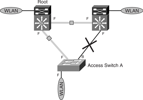**Figure 6-18** _STP Instances for Voice VLAN_  [Figure 6-19](https://learning.oreilly.com/library/view/building-resilient-ip/1587052156/ch06.html#ch06fig19) shows the topology of the wireless LAN virtual LAN (WLAN VLAN), which has the same uplink as that of the voice VLAN. 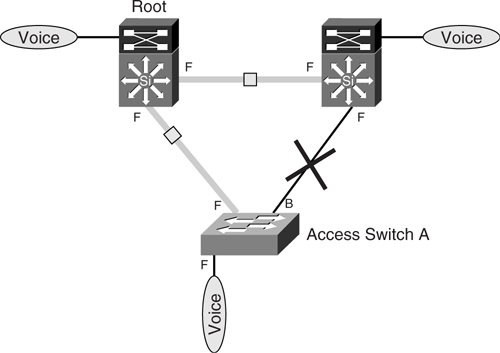**Figure 6-19** _STP Instances for WLAN VLAN_  Unlike the voice and WLAN VLANs, the data VLAN has been configured to use the other uplink. This design allows for load balancing of traffic between the VLANs. Whereas the voice and WLAN VLANs use the uplink on the left, the data VLAN uses the uplink on the right. [Figure 6-20](https://learning.oreilly.com/library/view/building-resilient-ip/1587052156/ch06.html#ch06fig20) shows the data VLAN topology. **Figure 6-20** _STP Instance of Data VLAN_  From an IP network perspective, regardless of the topology of the Layer 2 network, the logical IP networks of the three VLANs look exactly the same. The load balancing of traffic is achieved at a Layer 2 level and is transparent from an IP network perspective. The implication of this is that we have improved traffic-forwarding capability for all VLANs from switch A, utilizing both uplinks toward the distribution switches. In the event of a failure on any of the uplinks, all VLANs will be carried on the single remaining uplink. Because PVST has each VLAN governed by its own STP instance, it still operates within the confines of STP and may exhibit problems that are typical of a STP implementation. Therefore, the following features are available with the implementation of PVST: • PortFast • UplinkFast • BackboneFast • BPDUGuard • RootGuard • LoopGuard ##### Per-VLAN Spanning Tree Plus (PVST+) As mentioned in the preceding section, PVST gives you flexibility in creating a separate Layer 2 topology for each VLAN, thereby achieving Layer 2 load balancing toward the distribution layer. However, it runs only with the ISL trunking feature, not IEEE 802.1q. Per-VLAN Spanning Tree Plus (PVST+) was introduced so that a network with PVST can interoperate with a network that runs IEEE 802.1q. When you connect a Cisco switch to other vendors’ devices through an IEEE 802.1q trunk, PVST+ is deployed to provide compatibility. The following features are available with the implementation of PVST+: • PortFast • UplinkFast • BackboneFast • BPDUGuard • RootGuard • LoopGuard Although PVST and PVST+ give flexibility in terms of traffic distribution on the trunks, they tax the control planes of the switches implementing them. In both PVST and PVST+, each STP instance is a separate process and requires independent control a plane resources. Imagine if there are tens or hundreds of VLANs defined; there will be the same number of STP instances running in the switch. In the event of a topology change, these STP instances will have to go through the same steps to process the change. When this happens, the performance of the switch will be affected, and in some cases, no traffic can be forwarded at all because the control plane is overloaded. One solution to this is to implement 802.1s, which you learn about in the “[IEEE 802.1s](https://learning.oreilly.com/library/view/building-resilient-ip/1587052156/ch06.html#ch06sec2lev7)” section. #### IEEE 802.1w The IEEE 802.1d protocol was invented at a time when network downtime was not stringent at all. With the increase in networking speed and expectation of the network resiliency, the IEEE 802.1d protocol is finding it hard to keep up with the demand of the modern IP network. The enhancements discussed thus far have been Cisco proprietary enhancements, and interoperability with other vendors’ implementation may not be possible. IEEE 802.1w, or better known as Rapid Spanning Tree Protocol (RSTP), is the standard’s answer to all the enhancements discussed so far. The motivations for the development of 802.1w include the following: • Backward compatibility with the existing 802.1d standard • Doing away with the problem with respect to long restoration time in the event of a failure • Improvement in the way the protocol behaves, especially with respect to modern networking design Because 802.1w is an enhancement of the 802.1d standard, most of the concepts and terminology of 802.1d still apply. In addition, because it is backward compatible with the IEEE 802.1d standard, it is possible to interoperate with older networks that are still running the original protocol. As its name implies, the most important feature of 802.1w is its capability to execute transition rapidly. Whereas a typical convergence time for 802.1d is between 35 and 60 seconds, the 802.1w can achieve it in 1 to 3 seconds. In some cases, a subsecond convergence is even possible. The 802.1d protocol was slow in its operation because ports take a long time to move into a forwarding state. In 802.1d, the only way to achieve faster convergence is to change the value of the Forward Delay and Maximum Age timers. Even then, it is still a timer-based protocol. The 802.1w can achieve faster convergence because it can move a port to a forwarding state without waiting for any timer to expire. 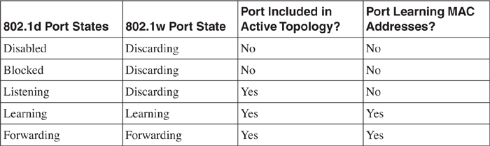It does so via a few new features: • New port roles and states • New BPDU format and handshake mechanism • New edge port concept • New link type concept In the original 802.1d standard, a bridge port may be in one of the five possible states: disabled, blocked, listening, learning, or forwarding. 802.1w reduces the port states to three: discarding, learning, and forwarding. [Table 6-2](https://learning.oreilly.com/library/view/building-resilient-ip/1587052156/ch06.html#ch06tab02) compares the port states of the two standards. **Table 6-2** _Comparison of 802.1d and 802.1w Port States_  In the original 802.1d standard, a port can take on the role of a root, designated, or alternate. In the 802.1w, a port can take on a root, designated, alternate, or backup role. [Table 6-3](https://learning.oreilly.com/library/view/building-resilient-ip/1587052156/ch06.html#ch06tab03) compares the port role of the two standards. 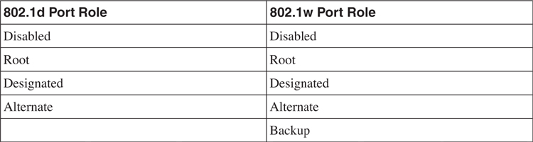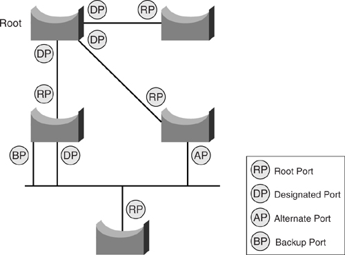**Table 6-3** _Comparison of 802.1d and 802.1w Port Roles_  In 802.1w, an alternate port is one that receives preferred BPDUs from other bridges, whereas a port is designated as backup if it has received preferred BPDUs from the same bridge that it is on. [Figure 6-21](https://learning.oreilly.com/library/view/building-resilient-ip/1587052156/ch06.html#ch06fig21) illustrates the concept of the new port roles. **Figure 6-21** _Port Roles of IEEE 802.1w_  The format of the 802.1w BPDU differs from that in 802.1d. In 802.1d, only the Topology Change (TC) and Topology Change Acknowledgement (TCA) were defined. In the new standard, the rest of the 6 bits are used to include the following flags: • Proposal • Port Role (2 bits) • Learning • Forwarding • Agreement The inclusion of the new flags enables the bridges to communicate with each other in a new manner. In the 802.1d standard, BPDUs are propagated via a relay function. In other words, the root bridge sends out BPDUs and the rest will relay the message to the downstream. Unlike 802.1d, 802.1w uses Hello packets between bridges to maintain link states and does not rely on the root bridge. In 802.1w, bridges send out BPDUs to their neighbors at fixed times, as specified by the Hello timer. When a bridge has not received a BPDU from its neighbor, it can assume that its neighbor is down. This reliance on Hello packets, rather than the Forward Delay and Maximum Age timers in the original 802.1d, enables the bridges to perform notification and react to topology change in a much more efficient manner. In 802.1w, the edge port refers to a port that is directly connected to an end station. Because an end station is not a bridge and will not cause loops, the port can be put into a forwarding state immediately. This is exactly the same concept as that of the PortFast feature in the Cisco implementation. An edge port does not cause topology change, regardless of its link state. However, if it starts to receive BPDUs, it will lose its edge port status and become a normal STP port. The advent of switching technology has resulted in changes to network design. Nowadays, switches are connected more in a point-to-point manner than through shared media. By taking advantage of the point-to-point link’s characteristics, 802.1w can move a port into forwarding state much faster than before. The link type is derived from the duplex mode of the port. A link connected via a full-duplex port is considered to be point to point, whereas one that is connected via a half duplex is considered to be shared. The link type can also be configured manually in 802.1w. Therefore, a simple configuration of a port mode now significantly affects the behavior of the STP. The 802.1w is made available on the Catalyst switches through the implementation of Rapid-PVST+. Rapid-PVST+ enables you to load balance VLAN traffic and at the same time provide rapid convergence in the event of a failure. 802.1w is also incorporated into the Cisco implementation of IEEE 802.1s. IEEE 802.1s is discussed in the following section. [Example 6-11](https://learning.oreilly.com/library/view/building-resilient-ip/1587052156/ch06.html#ch06ex11) shows how to turn on Rapid-PVST+ in the global configuration mode. **Example 6-11** _Configuring Rapid-PVST+_ --- 3750-A#configure terminal 3750-A(config)#spanning-tree mode rapid-pvst --- Because 802.1w has introduced a few enhancements to the original 802.1d, not all features discussed in the section “[The Spanning Tree Protocol: IEEE 802.1d](https://learning.oreilly.com/library/view/building-resilient-ip/1587052156/ch06.html#ch06sec2lev4)” are needed. The following features are available in conjunction with Rapid-PVST+: • PortFast • BPDUGuard • RootGuard • LoopGuard As mentioned earlier, the 802.1w protocol can work with the 802.1d protocol to provide interoperability. However, all the 802.1w enhancements are lost, and the behavior will be that of the original standard. #### IEEE 802.1s The IEEE 802.1s protocol is another standard that deals with mapping VLAN topology with an independent instance of STP. To have a good understanding of IEEE 802.1s, you have to appreciate the differences between the CST model and PVST model. In the deployment of CST, only one instance of STP is running in the switches, and as a result, all VLANs share the same Layer 2 topology. The characteristics of a CST implementation are as follows: • Only one instance of STP is running for all VLANs; therefore, the CPU load on the switches is minimal. • Because all VLAN topologies are governed by the same STP process, they all share the same forwarding path and blocked path. • No load balancing of traffic is permitted. By adopting a PVST strategy, you can achieve a different implementation, such as that shown earlier in [Figure 6-17](https://learning.oreilly.com/library/view/building-resilient-ip/1587052156/ch06.html#ch06fig17), with the following characteristics: • Each VLAN is governed by a separate STP instance. Because of this, the CPU load on the switch has increased. With a network of 1000 VLANs, there are actually 1000 instances of STP running. • Because each VLAN has its own STP instance, they can be configured differently to achieve different Layer 2 topology. • Load balancing of traffic is achieved via configuration. • There will be many VLANs sharing the same Layer 2 topology, and each VLAN will have its own STP instance. Both of the preceding implementations have their pros and cons. CST achieves saving on CPU resources but sacrifices on topology flexibility and load-balancing capability. PVST sacrifices CPU resources to achieve better control of the topology and uplink capacity. The IEEE 802.1s standard aims to combine the benefits of the two implementations. The idea behind the IEEE 802.1s standard is to map those VLANs that share the same topology to a common instance of STP. This way, you can reduce the number of instances of STP running, thus reducing the load on the CPU. At the same time, other VLANs may be mapped to another instance of STP for a different topology. This way, the flexibility of topology is made possible and load balancing can be achieved. In [Figure 6-22](https://learning.oreilly.com/library/view/building-resilient-ip/1587052156/ch06.html#ch06fig22), both voice and data VLANs are mapped to STP instance 1, where the uplink on the right is blocked. On the other hand, as illustrated in [Figure 6-23](https://learning.oreilly.com/library/view/building-resilient-ip/1587052156/ch06.html#ch06fig23), the WLAN VLAN is mapped to STP instance 2, where the uplink on the left is blocked. 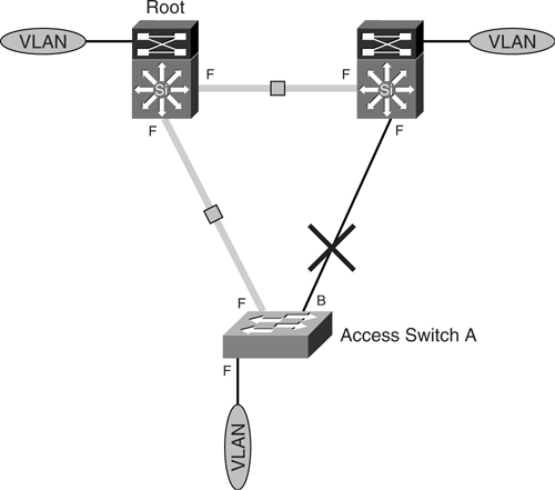**Figure 6-22** _STP Instances of IEEE 802.1s for Voice and Data VLANs_  **Figure 6-23** _STP Instances of IEEE 802.1s for WLAN VLANs_  All in all, there are two instances of STP governing the topology of the three VLANs. With this implantation, it is possible to have, for example, 500 VLANs mapped to STP instance 1 and another 500 VLANs mapped to STP instance 2. Without 802.1s running, you need 1000 instances of STP running in the switch. The benefit of the IEEE 802.1s is in saving CPU resources from managing too many STP instances. However, the drawback is that it adds complexity to the network design. Keeping track of which VLAN is mapped to which STP instance may be an administrative burden. [Example 6-12](https://learning.oreilly.com/library/view/building-resilient-ip/1587052156/ch06.html#ch06ex12) shows an 802.1s configuration. The Catalyst series switches support a maximum of 16 instances of RSTP. Note that RSTP is enabled by default when you configure 802.1s. **Example 6-12** _Configuring 802.1s_ --- 3750-A#configure terminal 3750-A(config)#spanning-tree mst configuration 3750-A(config-mst)#instance 1 vlan 5-10 3750-A(config-mst)#name HRServers 3750-A(config-mst)#revision 1 3750-A(config-mst)#exit 3750-A(config)# --- The following error-prevention features are still made available to the instances of STP within 802.1s: • PortFast • BPDUGuard • RootGuard • LoopGuard In the Catalyst series of switches, the 802.1s feature is implemented together with the 802.1w. Therefore, its implementation is not only capable of saving control-plane resources but also converging in subseconds in some cases. 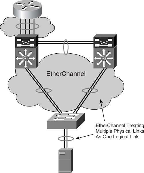#### Channeling Technology The channeling technology enables you to use multiple Ethernet links combined into one logical link. This configuration allows for increments in transmission capability between devices and provides link redundancy. It can be used to interconnect LAN switches or routers and even improves the resiliency of a server connection to a switch. The Cisco implementation of channeling technology is the EtherChannel. Depending on the connection speed, EtherChannel is referred to as Fast EtherChannel (FEC) for 100-Mbps links or Gigabit EtherChannel (GEC) for 1-Gbps links. The EtherChannel for 10-Gbps links is also available today. [Figure 6-24](https://learning.oreilly.com/library/view/building-resilient-ip/1587052156/ch06.html#ch06fig24) shows the basic concept of EtherChannel. **Figure 6-24** _EtherChannel_  EtherChannel operation comprises two parts: • The distribution of data packets on the multiple physical links • A control portion that governs the working of the technology The distribution of the packets is based on a hashing algorithm that derives a numeric value to decide which links to send the packet to. The algorithm may decide on the distribution based on the following: • Source MAC address • Destination MAC address • Source/destination MAC address • Source IP • Destination IP • Source/destination IP • Source TCP port • Destination TCP port • Source IP/destination IP/TCP port Based on the distribution criteria, the hashing is deterministic, and all packets that share the same characteristics are always transmitted via the same physical link to avoid sequencing errors. Depending on the hardware architecture, not all the Cisco devices support the algorithm. The control portion of the EtherChannel governs the working of the EtherChannel. There are three ways to bring up EtherChannel: • Manual configuration • Port Aggregation Control Protocol (PAgP) • IEEE 802.1ad, also known as Link Aggregation Control Protocol (LACP) Before participating in the channeling operation, a port can be in one of the EtherChannel modes listed in [Table 6-4](https://learning.oreilly.com/library/view/building-resilient-ip/1587052156/ch06.html#ch06tab04). 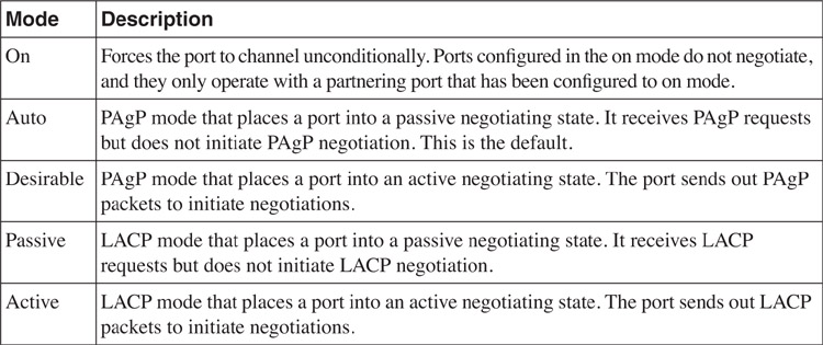**Table 6-4** _Different Modes of EtherChannel_  The manual way to configure EtherChannel dictates that both ports must be set to on to form the EtherChannel. The PAgP supports the autocreation of EtherChannel by the exchange of the PAgP packets between ports. This happens only when the ports are in auto and desirable modes. The basic rules for PAgP are as follows: • A port in desirable mode can form an EtherChannel with another port in desirable mode. • A port in desirable mode can form an EtherChannel with another in auto mode. • A port in auto mode cannot form an EtherChannel with another also in auto mode, because neither one will initiate negotiation. Likewise, the LACP supports the autocreation of EtherChannel by the exchange of the LACP packets between ports. This happens only when the ports are in active and passive modes. The basic rules for LACP are as follows: • A port in active mode can form an EtherChannel with another port in active mode. • A port in active mode can form an EtherChannel with another in passive mode. • A port in passive mode cannot form an EtherChannel with another also in passive mode, because neither one will initiate negotiation. Channeling technology is a good way to increase link capacity, provide link redundancy, and at the same time maintain the logical design of the IP network. However, care should be taken when deploying channeling technology, as discussed in the following section. #### Layer 2 Best Practices The health of the Layer 2 network plays an important role in maintaining the stability of the IP network within the access module. However, it is a common source of network error, with problems ranging from broadcast storms to complete network meltdowns. However, by following some simple principles, you can avoid these problems. ##### Simple Is Better It cannot be stressed enough that in the Layer 2 network design, simple is more, and more may not be beautiful. What this means is that you have to keep the design as simple as possible, with easy-to-remember configuration settings. The following are some examples: • If there is no uplink congestion problem, there is no need to load balance traffic. • In the event that you load balance traffic, choose a simple formula. For example, the human resources (HR) department uses the left uplink as the primary path, and the finance department uses the right uplink as the primary path. Never try to formulate a complex web of tables just to keep track of which VLAN has the left uplink as primary and which has the right as primary. A common approach is to have VLANs with even VLAN IDs going to the left and VLANs with odd VLAN IDs going to the right. • If changing the bridge priority is enough, leave the path cost alone. By keeping the Layer 2 design simple, you can actually improve the resiliency and convergence of the network. Another benefit is that it will make troubleshooting a lot easier in the event of a problem. ##### Limit the Span of VLANs If possible, confine the span of the VLAN to a minimum. This means you should avoid building a VLAN that spans multiple access modules. Provided you are dealing with some legacy application that needs all hosts to be on the same subnet, there is no reason why you should build a campus-wide VLAN. Such a VLAN not only takes up too many resources to maintain topology, you will probably end up with a nonoptimized traffic path that uses bandwidth unnecessarily. In addition, when there is an STP problem within the VLAN, too many switches will be involved in the convergence exercise. This increases the chance of a network-wide outage and should be avoided. ##### Build Triangles, Not Squares Features such as UplinkFast and BackboneFast work best in a triangle topology—that is, a single access switch having dual uplinks to a pair of distribution switches. In some situations, access switches are daisy-chained via physical connections. With two access switches, you end up with a square topology. With more than two access switches, you end up with a ring architecture. Both the square and ring designs suffer from poorer convergence time in the event of a failure. Although RSTP may still achieve the desired convergence time, the resulting topology may be too difficult to manage and troubleshoot. 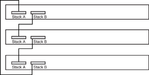If you have to daisy chain the access switches, you should consider the StackWise technology available on the Catalyst 3750. With StackWise technology, you can stack up to nine access switches and yet they are seen as one device from a Layer 2 and 3 perspective. From an STP perspective, they are viewed as one bridge, and from an IP network perspective, they can be managed via a single IP address. [Figure 6-26](https://learning.oreilly.com/library/view/building-resilient-ip/1587052156/ch06.html#ch06fig26) shows three Catalyst 3750s connected to each other via the StackWise technology. 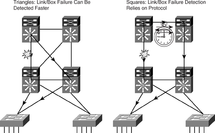**Figure 6-25** _Triangle and Square Topologies_  **Figure 6-26** _Connecting Catalyst 3750s via StackWise Technology_  ##### Protect the Network from Users The access module is where users have a direct connection to the network. You can never trust that only end stations such as PCs and laptops are connected to the access switches. The combination of users connecting a switch to the network and turning on the PortFast feature on that port could spell disaster for the STP topology. Therefore, the STP network has to be protected from all users via features such as BPDUGuard and RootGuard. You have to be cautious with the user-side connections to the network. Always imagine that users are going to put in technologies that are detrimental to the health of the network. ##### Selecting Root Bridges The root bridge is the most important component in the Layer 2 network. Its location within the Layer 2 topology and the selection of hardware impact the health of the Layer 2 network. Because all traffic in the Layer 2 network flows toward the root, the distribution layer switches are always good candidates. This corresponds to the way the IP traffic flows in the Layer 3 network. For redundancy purposes, there are usually two distribution switches per block, and they should be selected as the primary and secondary root bridge. Remember that in STP the bridge with the lowest BID is always elected as a root bridge. Therefore, you should not leave default values when configuring the BID of the switches. For this reason, part of the network design should include a BID assignment strategy. One common mistake that network managers make is to leave the operation of STP to the default values and behavior. The problem with this is that the selection of the root is not deterministic, and the resulting Layer 2 topology might not be optimized. Worse still, in the event of a problem, you have to determine the location of the root bridge. The most difficult problem to troubleshoot is a floating network design, where it is difficult to determine how it should work in the first place. You should decide on a root bridge and a backup root bridge so that the Layer 2 topology is fixed and easily understood. With proper configuration and documentation, traffic has to flow in a certain manner. This way, any anomaly can be easily identified and the problem diagnosed. The root bridge has to be protected via features such as RootGuard, and if it is possible, no access switch should be elected as a root bridge. Remember that the distribution layer is the most complex part of the access module, because it runs both Layer 2 and Layer 3 protocols. Therefore, the load on its control plane will be relatively higher than the rest of the switches in the network. For this reason, careful selection of hardware is important, and switches with higher-performance CPUs should be preferred. ##### Use Value-Added Features You can also use the **diameter** keyword to specify the Layer 2 network diameter (that is, the maximum number of switch hops between any two end stations in the Layer 2 network). When you specify the network diameter, the switch automatically sets an optimal Hello time, forward-delay time, and maximum-age time for a network of that diameter, which can significantly reduce the convergence time. You can use the **hello** keyword to override the automatically calculated Hello time. [Example 6-13](https://learning.oreilly.com/library/view/building-resilient-ip/1587052156/ch06.html#ch06ex13) shows a configuration sample of limiting the diameter to four switches for VLAN 100. **Example 6-13** _Setting the Diameter of a Layer 2 Network_ --- 3750#configure terminal 3750(config)#spanning-tree vlan 100 root primary diameter 4 --- ##### EtherChannel Deployment A common place to deploy EtherChannel is the connection between the distribution switches. Such a connection is usually configured as a switching trunk port, and, therefore, the bundling is called a Layer 2 EtherChannel. On the other hand, an EtherChannel may be deployed as a routed interface, such as that between a distribution layer switch and a core layer switch. Such an implementation is called a Layer 3 EtherChannel. Extra care has to be taken with the implementation of a Layer 3 EtherChannel because many advanced IP features, such as Multiprotocol Label Switching-Traffic Engineering (MLPS-TE), Reservation Protocol (RSVP), and QoS, with complex configurations may not be supported in conjunction with a Layer 3 EtherChannel. Different linecards on different platforms may have an individual caveat with respect to this scenario, and it is important that you are familiar with these caveats. Because of the potential complexity that Layer 3 EtherChannel may introduce in such a scenario, link capacity scaling and resiliency in the core module require a different approach than that provided by EtherChannel. ##### EtherChannel Load Balancing The default hashing algorithm for EtherChannel is based on the source/destination IP pair. This mode is adequate for most user access implementations. However, sometimes this might yield unexpected results. One good example is when a pair of servers is performing application synchronization. Because the source/destination IP pair remains constant throughout the transmission, you end up with only one of the links of an EtherChannel being utilized. This may have a performance impact if the transmission exceeds the transmission capacity of the single link. One good way to overcome this problem is to adopt the source IP/destination IP/TCP port hashing algorithm for the EtherChannel. Including Layer 4 information allows for a more balanced use of the available links within the EtherChannel bundle. ##### Consistent EtherChannel Port Settings When configuring EtherChannel, you have to ensure that all members of the bundle have the same port setting. This includes settings such as the link speed and duplex mode. If you have ports with different settings, you may face unexpected results and find troubleshooting more difficult. For example, ports belonging to the same EtherChannel configured with different trunking modes may produce undesirable STP behavior. All ports need to be in enabled mode, too. Having some ports in disabled mode will cause traffic to be diverted to the rest. ##### Layer 2 Setting for EtherChannel When setting up the Layer 2 EtherChannel, take care with respect to the Layer 2 setting. For example, if the EtherChannel is to act as a logical access port for VLAN 10, all the switch ports that make up the EtherChannel have to be set to the same VLAN. If the EtherChannel is to act as a logical trunk port, however, all the switch ports that make up the EtherChannel have to be in trunk mode. In addition, the allowed range of VLANs has to be the same for all the ports. Failing to ensure port setting consistencies means that the EtherChannel will never be formed. ##### Turning Off Autonegotiation Although the switches can autonegotiate for the formation of EtherChannel via protocols such as PAgP, it is better to configure them manually. For example, PAgP is on by default for switches running CatOS, whereas it is off by default for those running IOS. A mismatch PAgP setting can incur unnecessary negotiation time and may take a long time to restore connection. Turning off autonegotiation on ports between servers and switches is also a good idea to improve resiliency of the network. Some server network interfaces might not negotiate the link properly and cause duplex mismatch. The server network interface card may think that the switch port is running as a half duplex, when in fact the switch port is a full duplex. Therefore, it is always recommended to explicitly set the duplex settings on both the server interface and the switch port. So far, you have learned about all the Layer 2 building blocks that enable you to build a stable Layer 2 network. After the Layer 2 network is robust and has high resiliency, you can then build the corresponding IP subnets to be always reachable from other parts of the network. ### Layer 3 Domain The Layer 3 building block is found mainly in the distribution layer of the multilayer campus design. The function of the building block is mainly to provide for the following: • A first-hop redundancy function to the hosts that are attached to the access layer • To announce the routes of the IP subnet sitting behind the distribution layer to the rest of the network • Other value-added functions that may help in the operation of the network (for example, access control, multicast forwarding, and QoS) Because of the functions it provides, resiliency at the Layer 3 domain focuses on devices backing up each other in terms of providing all the previously described functions. #### Hot Standby Routing Protocol (HSRP) Most of the end devices such as PCs, laptops, and servers are usually configured with a single default IP gateway. What this means is that if the default IP gateway is unavailable, these devices cannot communicate beyond their subnet. Although a feature such as Router Discovery Protocol may help in looking for another default IP gateway, not many end devices support it. Therefore, ensuring the availability of the default IP gateway is a number one priority. 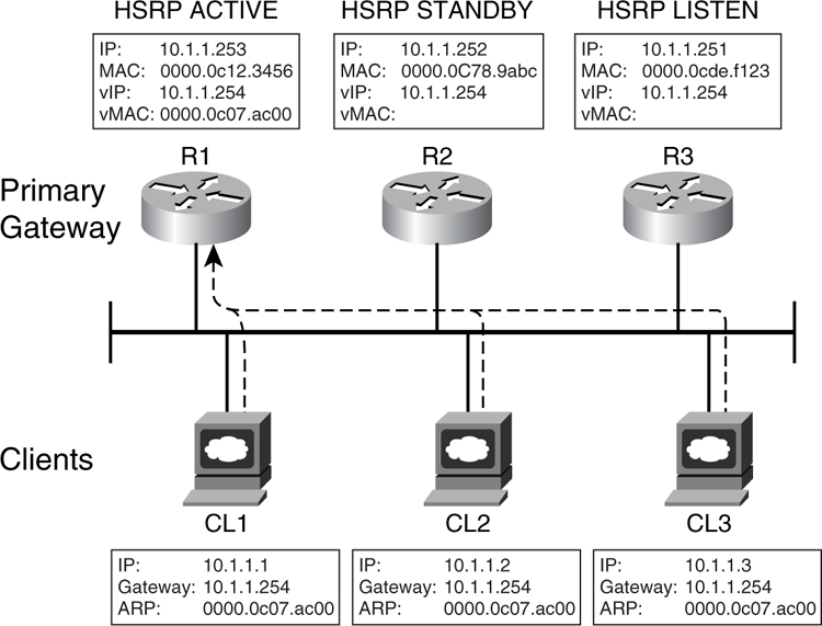The Hot Standby Routing Protocol (HSRP) is the Cisco implementation of providing a redundant default gateway to the end devices. Essentially, HSRP allows a set of routers to work together so that they appear as one single virtual default gateway to the end devices. It does so by providing a virtual IP (vIP) address and a virtual MAC (vMAC) address to the end devices. The end devices are configured to point their default IP gateway to the vIP address. The end devices also store the virtual vMAC address via Address Resolution Protocol (ARP). This way, HSRP allows two or more routers to back up each other to provide first-hop resiliency. Only one of the routers, the primary gateway, does the actual work of forwarding traffic to the rest of the network. There will be one standby router, whereas the rest will be placed in the listen mode. These routers do not forward traffic from the end hosts. However, for return traffic, they may forward traffic to the devices, depending on the configuration of the IP routing protocol. [Figure 6-27](https://learning.oreilly.com/library/view/building-resilient-ip/1587052156/ch06.html#ch06fig27) illustrates the concept of HSRP. When a router participates in a HSRP setup, it exchanges keepalive Hellos with the rest using User Datagram Protocol (UDP) packets via a multicast address. 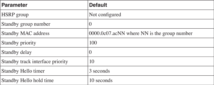**Figure 6-27** _HSRP_  [Table 6-5](https://learning.oreilly.com/library/view/building-resilient-ip/1587052156/ch06.html#ch06tab05) lists the default configuration values of the HSRP parameters. **Table 6-5** _Default Values for HSRP Configuration_  Here are some pointers about configuring HSRP: • The role of primary and standby routers can be selected by assigning a priority value. The default value of the priority is 100, and its range is 0 to 255. The router with the highest priority is selected as the primary, whereas zero means the router will never be the primary gateway. In the event that all the routers have the same priority, the one with the highest IP address is selected as the primary router. • The priority of the router changes if it has a standby track command configured and is brought into action. The tracking value determines how much priority is decremented when a particular interface that the router tracks goes down. A typical interface that is being tracked is the uplink toward the backbone. When the uplink toward the backbone fails, no traffic can leave the router. Therefore, the primary router should relinquish its role and have its priority lowered so that the standby router can take over its role. • You can track multiple interfaces, and their failure has a cumulative effect on the priority value of the router, if it has a track interface priority configured. If no track priority value is configured, the default value is 10, and it is not cumulative. • The default Hello timer is 3 seconds, whereas the hold time is 10 seconds. Hold time is the time taken before the standby declares the primary as unavailable when no more Hello packets are received. From an IP resiliency standpoint, the focus is on how fast the standby gateway router takes over in the event that the primary gateway is down. Note that this is only for traffic going out from the end devices toward the rest of the network. The downtime experienced by the end devices will be the time it takes for the standby router to take over. Although the standby router has taken over, its immediate neighbors may still keep the original primary router as the gateway to reach the access network. This happens because their routing tables have not been updated. In this case, for these routing tables to be updated, the routing protocol has to do its job. The default Hello timer for HSRP is 3 seconds, and the hold time is 10 seconds. This means that when the primary router is down, end devices cannot communicate with the rest of the network for as long as 10 seconds or more. The Hello timer feature has since been enhanced so that the router sends out Hellos in milliseconds. With this enhancement, it is possible for the standby router to take over in less than a second, as demonstrated in [Example 6-14](https://learning.oreilly.com/library/view/building-resilient-ip/1587052156/ch06.html#ch06ex14). **Example 6-14** _Configuring HSRP Fast Hello_ --- Router#configuration terminal Router(config)#interface fastEthernet 1/1 Router(config-if)#ip address 10.1.1.253 255.255.255.0 Router(config-if)#standby 1 ip 10.1.1.254 Router(config-if)#standby 1 timers msec 200 msec 750 Router(config-if)#standby 1 priority 150 Router(config-if)#standby 1 preempt Router(config-if)#standby 1 preempt delay minimum 180 --- In [Example 6-14](https://learning.oreilly.com/library/view/building-resilient-ip/1587052156/ch06.html#ch06ex14), the router R1 has been configured with a virtual IP address of 10.1.1.254, and its priority is 150. For R1 to be the primary router, the rest will have a default priority value of 100. R1 sends out a Hello packet every 200 ms with a hold time of 750 ms. The function of the **preempt** command allows R1 to take over the forwarding function after it has recovered from its error, or after it has been reloaded. The preempt delay timer is to force R1 to wait for the indicated amount of time, in this case 180 seconds, before claiming back its role. This is to prevent it from taking over the HSRP primary role without a proper routing table. Up to this point, HSRP may not seem like an efficient solution, because only one router, R1, is performing the forwarding function. The rest of the routers are simply not used at all. This might not even be a cost-effective solution, especially if all the HSRP routers are WAN routers with expensive WAN links as their uplinks. Because only the primary router is forwarding traffic, the rest of the WAN links on R2 and R3 will be left underutilized. The Multigroup HSRP (MHSRP) feature is used to solve this problem. You can configure MHSRP on a pair of routers. Both the routers R1 and R2 are configured with multiple HSRP groups. For each of the HSRP groups, there is a unique virtual IP address with a virtual MAC address. Group 1 has R1 as the primary router and R2 as the standby. Group 2 has R2 as the primary and R1 as a standby. The end devices are separated into groups by configuring their default gateway to point to the different virtual IP addresses. Half the end devices will default the route to group 1’s virtual IP address; the rest will default the route to group 2’s virtual IP address. [Figure 6-28](https://learning.oreilly.com/library/view/building-resilient-ip/1587052156/ch06.html#ch06fig28) illustrates the concept. 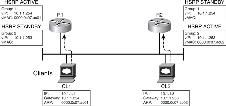**Figure 6-28** _MHSRP_  In this case, both the uplinks of R1 and R2 are utilized, because both are acting as the primary router for separate HSRP groups. Whenever the primary router of a group fails, the standby for that group takes over the duty of forwarding traffic. [Example 6-15](https://learning.oreilly.com/library/view/building-resilient-ip/1587052156/ch06.html#ch06ex15) shows the configuration needed for R1. **Example 6-15** _Configuration of HSRP on R1_ --- R1#configuration terminal R1(config)#interface ethernet1/0 R1(config-if)#ip address 10.1.1.250 255.255.255.0 R1(config-if)#standby 1 preempt R1(config-if)#standby 1 ip 10.1.1.254 R1(config-if)#standby 1 track Serial0 R1(config-if)#standby 2 ip 10.1.1.253 R1(config-if)#standby 2 track serial 0 R1(config-if)#standby 2 priority 95 --- [Example 6-16](https://learning.oreilly.com/library/view/building-resilient-ip/1587052156/ch06.html#ch06ex16) shows the configuration needed for R2. **Example 6-16** _Configuration of HSRP on R2_ --- R2#configuration terminal R2(config)#interface ethernet1/0 R2(config-if)#interface ethernet1/0 R2(config-if)#ip address 10.1.1.251 255.255.255.0 R2(config-if)#standby 1 ip 10.1.1.254 R2(config-if)#standby 1 track Serial0 R2(config-if)#standby 1 priority 95 R2(config-if)#standby 2 preempt R2(config-if)#standby 2 ip 10.1.1.253 R2(config-if)#standby 2 track serial 0 --- MHSRP solves the problem of wasted uplink bandwidth of the standby router in HSRP. However, it adds complexity because the clients now have to have separate default gateway addresses. If the clients have their IP address assigned by a DHCP server, some mechanism has to be built in to distribute the clients to point to different default gateways. In this case, you might have added complexity for the sake of load balancing traffic on the various uplinks. #### Virtual Router Redundancy Protocol (VRRP) The Virtual Router Redundancy Protocol (VRRP), which is defined in RFC 2338, is the IETF standard version of a first-hop redundancy protocol. Its function is similar to that of HSRP. Routers participating in a VRRP setup are known as _VRRP routers_. These routers work together to provide what is known as a VRRP virtual router. There can be many virtual routers, each identified through a virtual router identifier (VRID). This is similar to the group ID assigned in MHSRP configuration. In a similar concept as that of HSRP, VRRP routers elect a master router based on a priority value. The master router then sends out advertisements to the rest of the participating routers for keepalive. The minimum value of the advertisement interval is 1 second. In this case, the take over timing may not be as fast as that provided by HSRP. With VRID, VRRP can also provide a load-sharing mechanism to utilize all uplinks. #### Global Load Balancing Protocol (GLBP) In providing a first-hop redundancy solution, both HSRP and VRRP implement the concept of a single primary and multiple secondary gateways. Under normal working conditions, only the primary is actively forwarding traffic for the hosts; the secondary is not. This is costly, especially when both the uplinks from the gateways are expensive WAN circuits. Suppose the primary gateway has never encountered any problems; the secondary gateway may be forgotten after some time, or worse still, its failure may not be noticed. MHSRP may be able to achieve a certain degree of load balancing for the uplinks; however, the complexity of configuring the end devices to have a different default IP gateway may outweigh the benefits. This is especially so if a DHCP is involved. Not many DHCP servers can assign a default IP gateway in a round-robin fashion. The aim of the Global Load Balancing Protocol (GLBP) is to provide the basic function of first-hop redundancy, and at the same time achieve load balancing in terms of uplinks. GLBP combines the benefits of both HSRP and MHSRP. In a GLBP setup, routers work together to present a common virtual IP address to the clients. However, instead of using a single virtual MAC address tied to a virtual IP address, different virtual MAC addresses are tied to a single virtual IP address. These different virtual MAC addresses are sent to different end devices through the ARP process. This way, different end devices forward traffic to the different virtual MAC addresses for forwarding to the rest of the network. In a GLBP setup, as shown in [Figure 6-29](https://learning.oreilly.com/library/view/building-resilient-ip/1587052156/ch06.html#ch06fig29), a router is elected to be the active virtual gateway (AVG). The AVG acts as the master of the group. In [Figure 6-27](https://learning.oreilly.com/library/view/building-resilient-ip/1587052156/ch06.html#ch06fig27), R1 has been elected as the AVG. The job of the AVG is to assign a virtual MAC address to each GLBP member. These members then become the active virtual forwarder (AVF) for that virtual MAC address. For example, R2 is an AVF for the virtual MAC 0007.b400.0102. The AVF is responsible for forwarding traffic that was sent to their virtual MAC address. Other members may be assigned as a secondary virtual forwarder (SVF) in case the AVF fails. In [Figure 6-29](https://learning.oreilly.com/library/view/building-resilient-ip/1587052156/ch06.html#ch06fig29), R3 is the SVF for R2. One important job of the AVG is to respond to all ARP requests sent out by the end devices. The end devices send out an ARP request for the common virtual IP address. The AVG assigns a different virtual MAC to different end devices based on a preset algorithm. It may be assigned the virtual MAC in a round-robin or weighted fashion. In this manner, all the clients share the same default gateway IP address, which resolves into different MAC addresses, depending on which AVF has been assigned. 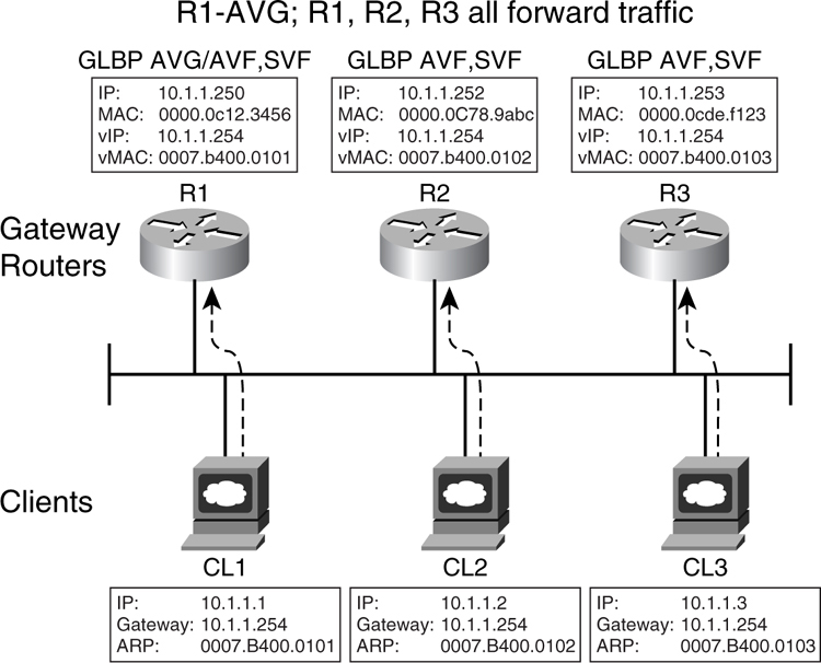**Figure 6-29** _GLBP_  The election of the AVG is the same as that of HSRP. The candidate is elected based on the **glbp priority** command. The one with the highest priority is elected the AVG. In the event of a tie, the one with the highest IP address is elected. There is another one elected as the standby; the rest are placed in listen mode. The members of the GLBP group communicate with each other via a multicast address 224.0.0.102 and UDP port number 3222. The virtual MAC address takes the form of 0007.b4nn.nnnn. The last 24 bits of the MAC address consists of six zeros, 10 bits for indicating the group number and 8 bits for the virtual forwarder number. This means GLBP can support 1024 groups, each with 255 forwarders. However, in practice, four virtual forwarders are configurable for each of the groups. The virtual forwarders are each assigned a virtual MAC address and act as the primary forwarder for that MAC address instance. The rest of the routers in the group learn of this virtual forwarding instance via Hello messages and create their own backup instance. These are known as the secondary virtual forwarders. The working of the primary and secondary forwarders depends on the four timers that are important in the GLBP operation: • **Hello time**—The Hello time is learned from the AVG, or it can be manually configured. The default is 3 seconds, and the range is 50 ms to 60 seconds. • **Hold time**—The hold time is used to determine whether action is required to take over the virtual gateway or virtual forwarder function. This timer is reset whenever a Hello is received from the partners. The hold time must be greater than three times that of the Hello timer. The hold time can be learned from the AVG or manually configured. The default is 10 seconds, and the range is 1 to 180 seconds. • **Redirect time**—This is the time in which the AVG continues to redirect clients to the AVF. The redirect time can be learned from the AVG or manually configured. The default is 5 minutes, and the range is 1 second to 60 minutes. • **Secondary hold time**—This is the period of time for which an SVF remains valid after the AVF is unavailable. The SVF is deleted when the secondary hold time expires. When the SVF is deleted, the load-balancing algorithm is changed to allocate forwarding to the remaining VFs. This timer should be longer than the ARP cache age of the client. This timer can be learned from the AVG or manually. The default is 1 hour, and the range is 40 minutes to 18 hours. There are three ways clients can be assigned to a particular virtual forwarder: • **Weighted load balancing**—The number of clients directed to an AVF depends on the weight assigned to it. All the virtual forwarders within a router use this weight. • **Host-dependent load balancing**—The decision of which AVF to direct to depends on the MAC address of the client. This way, a client is always directed to the same virtual MAC address. • **Round-robin load balancing**—As the name implies, the virtual MAC addresses are assigned to the clients in a round-robin fashion. This method is recommended for a subnet with a small number of clients. This is the default method. If no load-balancing algorithm is specified, the AVG responds to all ARP requests with its own VF MAC address. In this case, the whole operation is similar to that of HSRP. Similar to HSRP, GLBP can track interfaces. In fact, with the introduction of the Enhanced Object Tracking feature in Cisco IOS, GLBP can track and react to errors arising from the following entities: • Interfaces or subinterfaces • IP routes • All IP service level agreement (IP SLA) operations • Object lists via Boolean operations (for example, AND and OR) [Example 6-17](https://learning.oreilly.com/library/view/building-resilient-ip/1587052156/ch06.html#ch06ex17) shows how to configure GLBP on router R1. **Example 6-17** _Configuring GLBP on R1_ --- R1#configuration terminal R1(config)#interface fastethernet 0/0 R1(config-if)#ip address 10.1.1.250 255.255.255.0 R1(config-if)#glbp 10 ip 10.1.1.254 R1(config-if)#glbp 10 forwarder preempt delay minimum 60 R1(config-if)#glbp 10 load-balancing host-dependent R1(config-if)#glbp 10 preempt delay minimum 60 R1(config-if)#glbp 10 priority 254 R1(config-if)#glbp 10 timers 5 18 R1(config-if)#glbp 10 timers redirect 600 7200 --- GLBP combines the benefits of HSRP and MHSRP to achieve both first-hop resiliency and load balancing of traffic. It is especially important in a typical branch setup, which requires two WAN routers to provide a redundant setup. With GLBP, both the WAN links of the routers can be better utilized so that investment can be maximized. In addition, it is also good to use both links to verify their integrity. If a link is only used for redundancy purposes, it might not be possible to ascertain its quality until a failure has occurred. This may be too late. #### Layer 3 Best Practices This section looks at some Layer 3 best practices that focus on improving network resiliency. Besides providing a redundant first-hop gateway service to the access layer, another important task that the distribution layer has to perform is to provide robust IP connectivity for the access layer to the core layer. Besides providing a reroute capability in the event that a link for a device fails, the Layer 3 routing protocol can also provide load-balancing capability to achieve better throughput. ##### Adopt Topology-Based Switching Recall in the previous section, “[Layer 3 Domain](https://learning.oreilly.com/library/view/building-resilient-ip/1587052156/ch06.html#ch06sec1lev4),” that the Layer 3 building blocks are found in the distribution layer. This is where Layer 3 switching products are deployed to fulfill the role. In the selection of a Layer 3 switch, it is important to note that the switching hardware architecture does have a bearing on the resiliency of the IP network. [Figure 6-30](https://learning.oreilly.com/library/view/building-resilient-ip/1587052156/ch06.html#ch06fig30) shows a switching product that is based on flow-based architecture. In this architecture, the switch forwards traffic by sending the first packet of a traffic flow to the CPU. The CPU determines the outgoing port so that all subsequent packets are switched via hardware. The CPU also keeps a record of this flow in a hardware cache. In this architecture, the first packet of every flow involves the CPU of the switch. Flow-based architecture is a popular way to build a Layer 3 switch and can be found in many products on the market today. 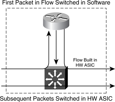**Figure 6-30** _Flow-Based Switching Architecture_  The problem with flow-based architecture is that every traffic flow is maintained in the cache, and this takes up memory. For a Layer 3 switch performing the role at the distribution layer, it can potentially be supporting hundreds and even thousands of hosts. These hosts can create huge numbers of flows that need to be maintained in the cache. With hosts entering and leaving the network over time, huge amounts of CPU and memory resources are needed to maintain the cache. This strain on the control-plane resources is most pronounced when there is a DoS attack on the distribution layer. With a flow-based architecture, it will quickly run out of resources trying to maintain the millions of flows that were generated by the attack. The resiliency of the entire distribution building block will be jeopardized in this scenario, because the control plane has run out of resources. In contrast to a flow-based architecture, a topology-based switching architecture is another way to build a Layer 3 switch. As discussed in the section “[Cisco Express Forwarding](https://learning.oreilly.com/library/view/building-resilient-ip/1587052156/ch03.html#ch03sec2lev12)” in [Chapter 3](https://learning.oreilly.com/library/view/building-resilient-ip/1587052156/ch03.html#ch03), “[Fundamentals of IP Resilient Networks](https://learning.oreilly.com/library/view/building-resilient-ip/1587052156/ch03.html#ch03),” CEF is an example of a topology-based switching architecture. [Figure 6-31](https://learning.oreilly.com/library/view/building-resilient-ip/1587052156/ch06.html#ch06fig31) shows the concept of a topology-based switching architecture. In this architecture, the CPU first builds the Forwarding Information Base (FIB) and adjacency table and pushes the information down to the ASIC in the line cards. Based on this information, the line card hardware can then forward traffic without the intervention of the CPU. With topology-based switching architecture, the CPU and its memory have been moved out of the way of all the traffic flows. Therefore, regardless of the number of hosts entering and leaving the network, the control plane of the distribution layer is not affected. Provided the DoS attack is targeted at the Layer 3 switch itself, the millions of flows that are created during the attack will have little impact on the control plane of the switch. 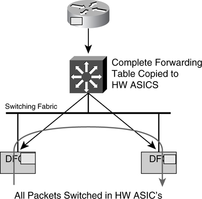**Figure 6-31** _Topology-Based Switching Architecture_  Therefore, a Layer 3 switch with a topology-based architecture is recommended to perform the role of the distribution layer. This is especially so if the Layer 3 switch is also to be used as in the core layer. Switches that incorporate topology-based architecture include the Catalyst 4500 and Catalyst 6500 series. ##### Using Equal-Cost Multipath It is important to understand the routing protocol behavior with respect to topology so that you can exploit certain characteristics to achieve resiliency. Because protocols such as Open Shortest Path First (OSPF) and Intermediate System to Intermediate System (IS-IS) work on the basis of path cost, you should always try to strive for a equal-cost multipath (ECMP) topology. It just means trying to create a topology with at least two equal-cost paths between a source and a destination. An ECMP topology allows traffic to be load balanced on multiple paths, thus achieving better performance. In addition, in the event that one of the paths fails, ECMP can transfer traffic to the remaining working path in an instant. One simple rule to remember about constructing an ECMP environment is that triangular topology is always preferred, the same as in the Layer 2 network design. In addition, it is also important to know how the router behaves in an ECMP environment. In an ECMP environment, the router takes advantage of the multiple links and tries to load balance traffic based on two algorithms: per destination or per packet. With per-destination load balancing, the router sends packets destined on the same path. Unequal use of the multiple paths may occur if most traffic is bound for one particular host. For example, only two hosts are communicating, and they are sending out a huge amount of traffic. However, with more hosts receiving traffic, the multiple paths are better utilized. Prior to CEF, the route cache was used to maintain the distribution of traffic across the multiple paths for these hosts. And the router had to build an entry for every host. This may also be a strain on the control plane of the router. With per-packet load balancing, the router sends packets across all the multiple paths in a round-robin fashion, which is a more balanced use of the multiple paths. Prior to CEF, this was done through process switching, and, therefore, this feature suffers from performance penalty. Recall from the section “[Cisco Express Forwarding](https://learning.oreilly.com/library/view/building-resilient-ip/1587052156/ch03.html#ch03sec2lev12)” in [Chapter 3](https://learning.oreilly.com/library/view/building-resilient-ip/1587052156/ch03.html#ch03) that CEF takes advantage of the separation between the forwarding table and the adjacency table to provide a better form of packet routing technology. With CEF, for per-destination load balancing, it does not need to build a cache entry for every host that needs load balancing. This frees up the control-plane resources and is especially important in building a resilient IP network. For per-packet load balancing, CEF does not need the help of the CPU to determine the next path for a packet to take. So there is minimal impact to the CPU load. Therefore, to fully take advantage of the benefits of a multipath topology, you need a good understanding of the load balancing algorithms and their impact on the load on the control plane. CEF is again recommended for the implementation of an ECMP environment. ##### Conserve Peering Resources The distribution layer terminates the VLANs coming from the access layer. Chances are, devices residing within these VLANs are end stations such as PCs or servers. These end stations rely on a default gateway to get connected to the rest of the network and do not normally run routing protocols. In this case, there is no need for the distribution layer to maintain any Layer 3 peering relationships with the devices in the VLANs. Cutting down on unnecessary peering will help conserve CPU and memory resources on the distribution layer switch, as shown in [Figure 6-32](https://learning.oreilly.com/library/view/building-resilient-ip/1587052156/ch06.html#ch06fig32). 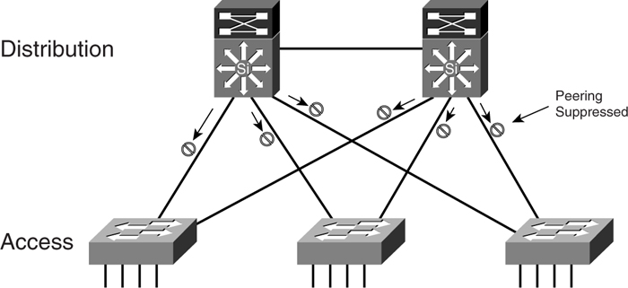**Figure 6-32** _Limiting Peering at the Distribution Level_  ##### Adopt a Hierarchical Addressing Scheme A basic rule that always holds true is this: The fewer the routes in the network, the faster it can converge. Therefore, it is worthwhile to adopt a hierarchical IP addressing scheme. A proper IP addressing scheme enables you to design the network in a hierarchical manner, where the routing table in the core should be less than that at the edge of the network. In conjunction with concepts such as areas in the OSPF protocol, IP addresses at the edge of the network can be summarized and represented by a single entry in the core. There are at least two advantages in doing so. First, because of the area design, errors such as link failure are concealed from the rest of the network. The error messages are propagated only within the area. Second, when errors occur within the area, no changes are required in the routing table for routers in other areas, because the summarized entry is still valid. As long as there are minimal changes to the routing table, the network will always remain stable. [Figure 6-33](https://learning.oreilly.com/library/view/building-resilient-ip/1587052156/ch06.html#ch06fig33) illustrates the concept of using areas in OSPF. 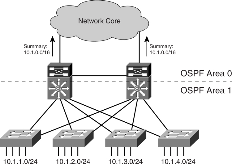**Figure 6-33** _Summarization in OSPF_  ### Summary The access module deals mainly with Ethernet switch technology. As long as the intricacy of the STP protocol is well understood, it is possible to build a robust Layer 2 network in this module. Keeping the Layer 2 design simple and predictable is perhaps the best insurance for building a resilient IP network within the access module. The same principle applies to the Layer 3 domain. By adopting the best practices, you can improve the resiliency of the network and avoid unnecessary downtime. table of contents search Settings [Chapter 5. Core Module](https://learning.oreilly.com/library/view/building-resilient-ip/1587052156/ch05.html) Chapter 6. Access Module queue Building Resilient IP Networks [Chapter 7. Internet Module ](https://learning.oreilly.com/library/view/building-resilient-ip/1587052156/ch07.html)